Background

At Surfee, we are developing a PathTracer for Surfee to realistically render users' 3D models in a web environment. Modern PathTracers aim for physically accurate lighting calculations, but they are limited by the fact that insufficient sample counts often result in severe noise in the final output. The Surfee team experienced this same issue during development. To resolve this, we attempted to apply Importance Sampling to HDR Environment Maps to increase sampling efficiency, which resulted in significant noise reduction. In this article, we will minimize equations and use intuitive examples to make the explanation easily understandable, not just for graphics developers but for a wide audience.

HDR Environment Map

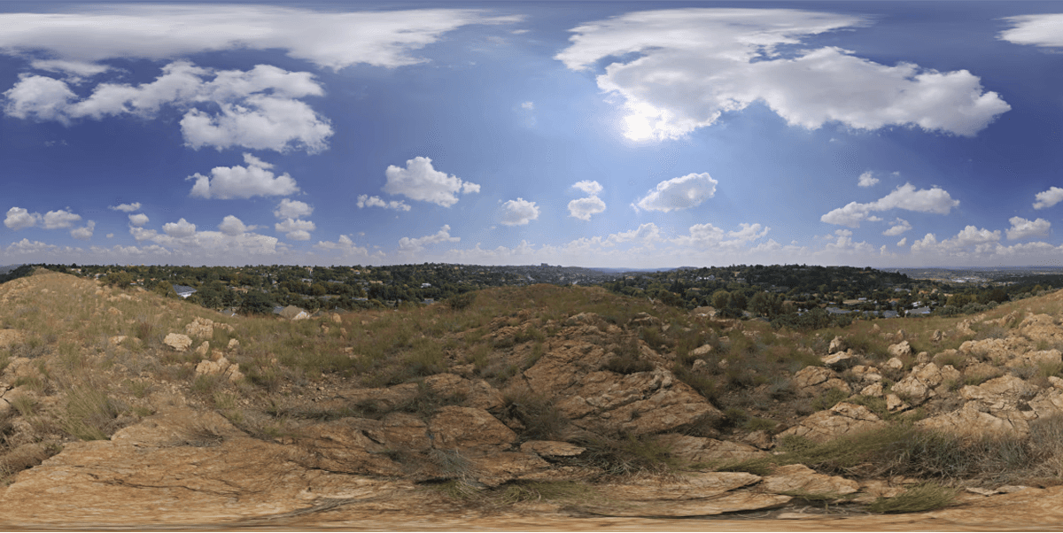
Environment Mapping is a technique for representing the surrounding lighting of a scene. Lighting is stored by mapping an Environment Map texture onto a sphere or cube surrounding the scene. Using an Environment Map allows for realistic lighting without having to manipulate individual light sources.

Environment Map

Environment Maps include LDR EnvMaps and HDR EnvMaps. The main difference between the two is the range of brightness they can store. While an LDR EnvMap can store a light range of 0 to 255 per pixel, an HDR EnvMap uses a 32-bit float type, allowing it to store extremely high light values. Therefore, using an HDR EnvMap enables the accurate distinction and representation of light differences between very bright areas (like the sun or artificial lights) and dark areas in the real world.

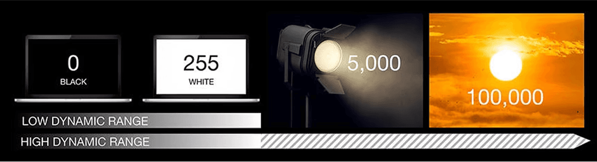
Comparison of brightness per pixel for HDR EnvMap and LDR EnvMap, What is a HDRI map?

Thus, the HDR EnvMap is an essential element for implementing realistic lighting quickly and efficiently in PathTracing. However, if used directly in a PathTracer, the HDR EnvMap can result in more severe noise than an LDR EnvMap. This is because most areas in an HDR EnvMap have relatively low brightness, with only small regions (like the sun in the example map) having very high brightness. Consequently, during sampling, the PathTracer often fails to adequately capture these small, very bright areas, leading to severe noise. Now, let's explore Importance Sampling, a technique for effectively sampling the HDR EnvMap.

Importance Sampling

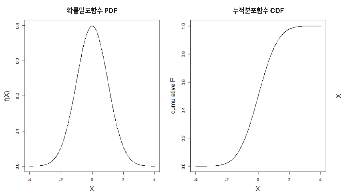
In the graph below, f(x) is the ideal sampling distribution (the correct answer), and pdf(x) is the probability of each sample occurring. If the pdf(x) graph is closely matched to f(x), noise will be reduced. The rightmost graph shows this form. The center graph represents uniform sampling, where all samples have the same probability, thus resulting in more noise than the rightmost graph. Our PathTracer before the improvement operated using this uniform sampling method, which led to high noise. Finally, we can expect the noise in the leftmost graph to be the largest, as important light sources are undersampled, while less important ones are oversampled.

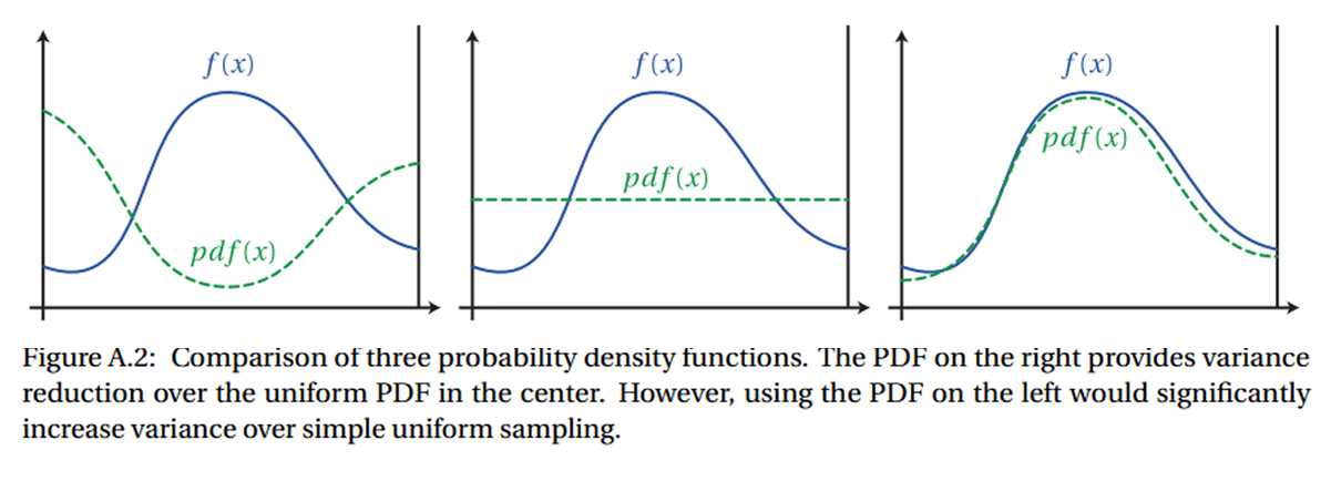
Efficient Monte Carlo Methods for Light Transport in Scattering Media, Wojciech Jarosz, Sep. 2008, Appendix A

Importance Sampling is a method that gives greater weight to the light in brighter pixels of the HDR EnvMap for sampling. In other words, it aligns the sampling probability with f(x), similar to the rightmost graph.

Importance Sampling has two types:

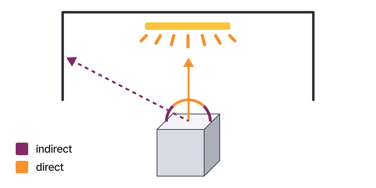
1. Final Bounce Sampling: Importance Sampling is performed on the determined ray path only if the ray travels to the final bounce and reaches the EnvMap. This is simpler to implement as it performs Importance Sampling only on the final bounce.

2. Next Event Estimation (NEE): Importance Sampling is performed at every bounce by directly sampling the light source. It accounts for the light source by casting a shadow ray in the sampled direction at every bounce to perform collision checking. While this increases the computational load, it reduces noise more effectively. This method is also referred to as Next Event Estimation (NEE).

Since the effects of the two Importance Sampling methods differ, both are generally applied in a PathTracer. Here, we will explain the more complex second method, Importance Sampling (NEE).

First, before performing Next Event Estimation, we must create data that reflects the EnvMap's pixel brightness:

• Marginal PDF: Weights for each row of the EnvMap.

• Conditional PDF: Weights for columns within a selected row of the EnvMap.

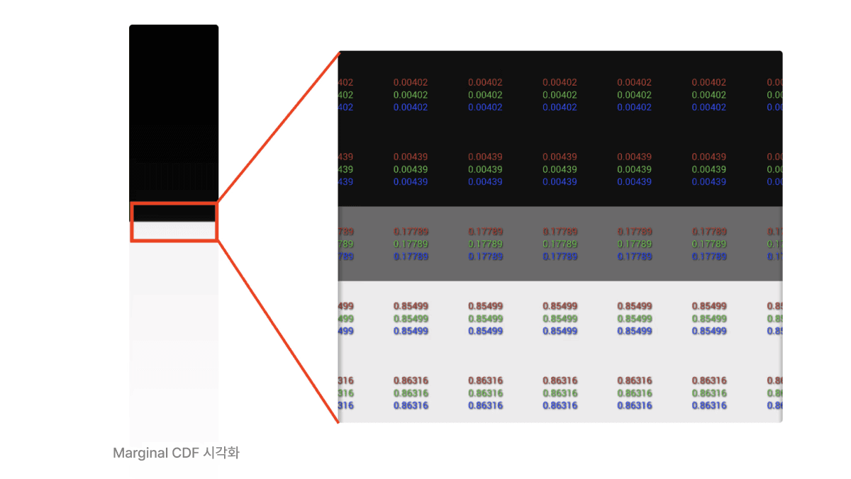
• Marginal CDF: Cumulative weights for each row of the EnvMap.

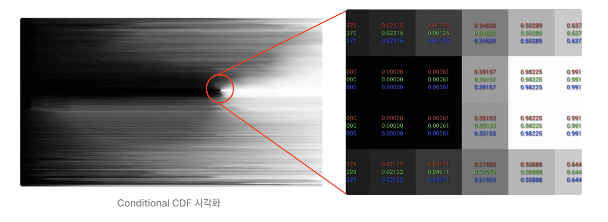
• Conditional CDF: Cumulative weights for columns within a selected row of the EnvMap.

The PDF (Probability Density Function) is a function that represents the probability of a continuous random variable taking a certain value. The probability must always be greater than or equal to 0, and the sum (integral) of the probabilities of all random variables equals 1.

The CDF (Cumulative Distribution Function) is, literally, the cumulative probability up to a certain random variable. Therefore, it represents the probability that a random variable will take a value less than or equal to x.

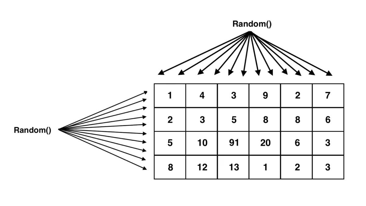
The grid in the figure below shows a very simplified EnvMap's pixels, with each pixel containing a light intensity value. The Marginal PDF/CDF represents the vertical light intensity weights of the EnvMap, and the Conditional PDF/CDF represents the horizontal light intensity weights.

First, let's find the Conditional PDF/CDF. The Conditional PDF/CDF is the column weight for a selected row, so it is stored in a 2D array with the size of EnvMap Width multiplied by Height. We sum all the pixels in each row to find the row-specific total light intensity. Then, by dividing the light intensity of each pixel by the row-specific total light intensity, we can find the probability (PDF) of each pixel. We can also find the CDF by accumulating the probabilities of each pixel from left to right. The remaining rows are calculated in the same way.

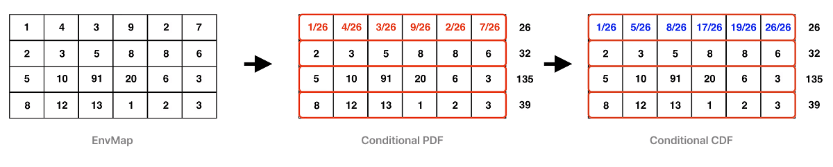
Conditional PDF/CDF Calculate

Next, let's find the Marginal PDF/CDF. The Marginal PDF/CDF contains the weights between the EnvMap rows, so it is stored in an array with the length of EnvMap Height. We have already calculated the total light intensity of each row above. We find the Marginal PDF by dividing each row's light intensity by the sum of all rows' light intensities. We also find the CDF by accumulating from the top.

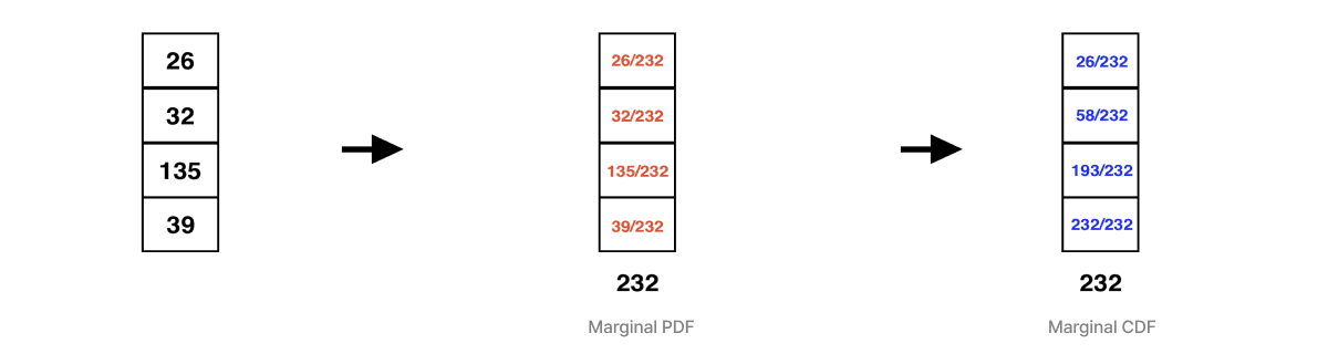
Marginal PDF/CDF Calculate

Now that the preparation for Importance Sampling is complete, we will explain how to use the CDF data to sample important light more frequently. Importance Sampling processes the rows first, then the columns of the EnvMap. We send a randomly chosen cumulative probability in the range 0.0-1.0 to the Marginal CDF to find the most important row among all the EnvMap rows. This part is very important.

To simplify, let's assume we randomly select target cumulative probabilities of 0.1, 0.2, 0.3, 0.4, 0.5, 0.6, 0.7, 0.8, 0.9, 1.0. We use binary search on the Marginal CDF to find the first index where the cumulative probability is greater than the target cumulative probability.

• 0.1 -> Index 0 (0.112)

• 0.2 -> Index 1 (0.25)

• 0.3 -> Index 2 (0.832)

• 0.4 -> Index 2 (0.832)

• 0.5 -> Index 2 (0.832)

• 0.6 -> Index 2 (0.832)

• 0.7 -> Index 2 (0.832)

• 0.8 -> Index 2 (0.832)

• 0.9 -> Index 3 (1)

• 1.0 -> Index 3 (1)

The binary search result shows that 6 out of 10 returned Index 2. This means that 6 out of 10 samples went to row 2 of the EnvMap. The size of the red arrows in the figure below visualizes the importance of each row. By calculating the pixel importance in the column direction in the same way, we can finally know which pixel's light is important during sampling. Finally, we can find the probability (PDF) that the final direction will actually be sampled.

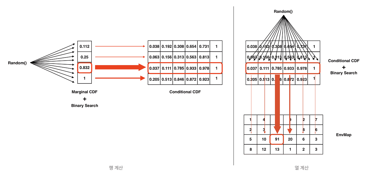
Importance Sampling

The existing method, as shown in the image below, unconditionally sampled EnvMap pixels randomly. This is why the noise was severe, as the light intensity of each pixel was not reflected.

Uniform Sampling

Now, let's calculate the Marginal CDF and Conditional CDF for a real EnvMap. This EnvMap has a very strong light source (the sun) in the middle when viewed vertically. Therefore, the Marginal CDF visualization image shows a rapid increase in the CDF around the middle.

Multiple Importance Sampling (MIS)

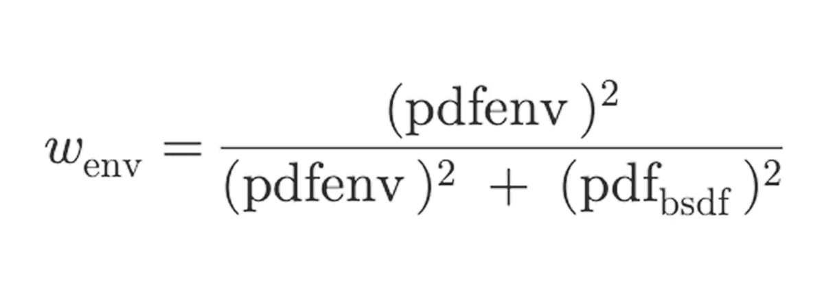
Above, we performed EnvMap Importance Sampling to find the probability (EnvMap PDF) that a specific direction would actually be sampled. We then mix the EnvMap PDF with the BSDF PDF that was calculated in the existing PathTracer using MIS. MIS is a technique that combines multiple sampling strategies to leverage the strengths and compensate for the weaknesses of each sampling. In MIS, the Power Heuristic formula shown below is generally used. This formula is derived experimentally and results in more BSDF samples being applied when the BSDF is more advantageous, and more EnvMap samples being applied when the EnvMap is more advantageous.

Application Results

Model: Car Scene	Model: Flight Helmet	Model: Persus

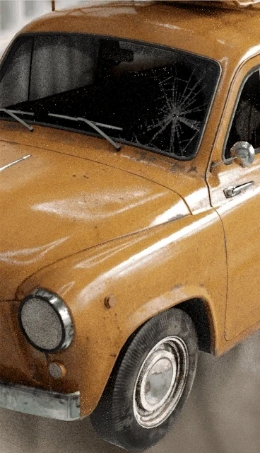
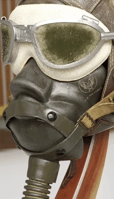
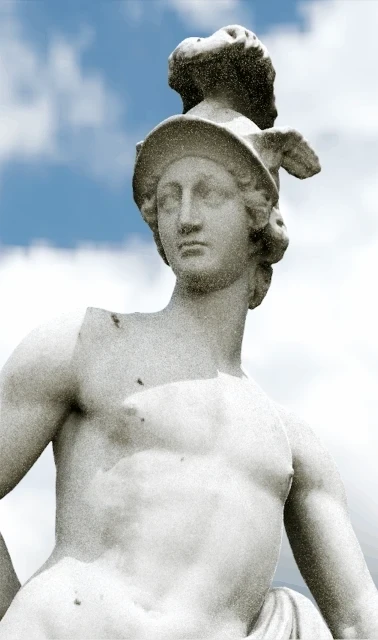
These images compare the results before and after applying Environment Map Importance Sampling (with 32 samples). All three comparison images show a significant overall reduction in noise. In the center helmet image, the noise is reduced enough to clearly recognize the patterns and text on the mask. And in the right statue image, the shadow cast by the sun overhead is also rendered realistically. Although Environment Map Importance Sampling adds the initial cost of weight calculation and the Scene Traversal cost for NEE execution, the quality improvement that can be expected is greater than these costs.

Average MSE reduction of 62.89% (in the 2 to 1024 spp range)

• MSE less than or equal to 20: 64 spp (MIS) compared to 256 spp (No-MIS) -> 4x sample savings

• MSE less than or equal to 10: 128 spp (MIS) compared to 1024 spp (No-MIS) -> 8x sample savings

Considerations for EnvMap Importance Sampling

Applying EnvMap Importance Sampling incurs initial costs for calculating pixel brightness-based weights (CDF/PDF). Additionally, individual lights such as Point, Area, and Spot lights must apply Importance Sampling in a different way than the EnvMap.

Future Work

To improve the quality of the PathTracer, we plan to sequentially implement the following tasks. Each technique aims to reduce noise.

• Adaptive Sampling: Reduce noise by actively adjusting the number of samples based on the degree of noise, rather than rendering the entire image with a uniform number of samples.

• Light MIS: MIS for individual light sources, in addition to the existing Environment Map MIS.

• Low-Discrepancy Samplers: Reduce noise by using low-discrepancy samplers such as Sobol, Halton, Stratified, and Blue Noise Samplers.

• Manifold Next Event Estimation (MNEE): Aim to improve noise in objects with refraction applied.

Conclusion

We have explored the overall process of introducing EnvMap Importance Sampling into a PathTracer to effectively reduce noise. We hope this article has helped you understand EnvMap Importance Sampling. We will continue to share interesting PathTracer-related topics. Furthermore, Surfee's proprietary PathTracer, which reflects these efforts, is scheduled to be deployed in Surfee this coming fall, so please look forward to it.

About the Author: Sejin Park Graphics Engineer, Surfee